


备注
点击 这里 下载完整示例代码
聊天机器人教程
Created On: Aug 14, 2018 | Last Updated: Jan 24, 2025 | Last Verified: Nov 05, 2024
在本教程中,我们探索了一个有趣的回归序列到序列模型的应用场景。我们将使用来自`Cornell Movie-Dialogs Corpus <https://www.cs.cornell.edu/~cristian/Cornell_Movie-Dialogs_Corpus.html>`__的电影脚本训练一个简单的聊天机器人。
对话模型是人工智能研究中的一个热点话题。聊天机器人可以在许多环境下找到应用,包括客户服务和在线帮助台。这些机器人通常由基于检索的模型驱动,这些模型根据某些形式的问题输出预定义的响应。在像公司IT帮助台这样高度受限的领域,这些模型可能足够,但它们对于更普通的应用场景来说还不够强大。教机器在多个领域与人类进行有意义的对话仍然是一项尚未解决的研究问题。近年来,深度学习的兴起使得像谷歌的`神经对话模型<https://arxiv.org/abs/1506.05869>`__等强大的生成模型成为可能,这标志着朝多领域生成对话模型迈出了重要的一步。在本教程中,我们将在PyTorch中实现这种模型。

> hello?
Bot: hello .
> where am I?
Bot: you re in a hospital .
> who are you?
Bot: i m a lawyer .
> how are you doing?
Bot: i m fine .
> are you my friend?
Bot: no .
> you're under arrest
Bot: i m trying to help you !
> i'm just kidding
Bot: i m sorry .
> where are you from?
Bot: san francisco .
> it's time for me to leave
Bot: i know .
> goodbye
Bot: goodbye .
教程亮点
处理和预处理`Cornell Movie-Dialogs Corpus <https://www.cs.cornell.edu/~cristian/Cornell_Movie-Dialogs_Corpus.html>`__数据集
实现一个带有`Luong注意力机制<https://arxiv.org/abs/1508.04025>`__的序列到序列模型
使用小批量共同训练编码器和解码器模型
实现贪婪搜索解码模块
与训练好的聊天机器人互动
致谢
本教程借鉴了以下资源的代码:
Yuan-Kuei Wu的pytorch-chatbot实现:https://github.com/ywk991112/pytorch-chatbot
Sean Robertson的practical-pytorch序列到序列翻译示例:https://github.com/spro/practical-pytorch/tree/master/seq2seq-translation
FloydHub Cornell Movie Corpus预处理代码:https://github.com/floydhub/textutil-preprocess-cornell-movie-corpus
准备工作
开始之前,`下载<https://zissou.infosci.cornell.edu/convokit/datasets/movie-corpus/movie-corpus.zip>`__电影对话语料库的zip文件。
# and put in a ``data/`` directory under the current directory.
#
# After that, let’s import some necessities.
#

import torch
from torch.jit import script, trace
import torch.nn as nn
from torch import optim
import torch.nn.functional as F
import csv
import random
import re
import os
import unicodedata
import codecs
from io import open
import itertools
import math
import json


# If the current `accelerator <https://pytorch.org/docs/stable/torch.html#accelerators>`__ is available,
# we will use it. Otherwise, we use the CPU.
device = torch.accelerator.current_accelerator().type if torch.accelerator.is_available() else "cpu"
print(f"Using {device} device")
加载和预处理数据
下一步是重新格式化数据文件并将数据加载到可以使用的结构中。
`Cornell Movie-Dialogs Corpus <https://www.cs.cornell.edu/~cristian/Cornell_Movie-Dialogs_Corpus.html>`__是一份丰富的电影角色对话数据集:
220,579条对话交换,涉及10,292对电影角色
来自617部电影的9,035名角色
总计304,713个语句
该数据集规模庞大且多样化,语言的形式、时间背景、情感等非常多样。我们希望这种多样性能使我们的模型应对多种形式的输入和查询。
首先,我们将查看数据文件中的一些行以了解原始格式。
corpus_name = "movie-corpus"
corpus = os.path.join("data", corpus_name)

def printLines(file, n=10):
    with open(file, 'rb') as datafile:
        lines = datafile.readlines()
    for line in lines[:n]:
        print(line)

printLines(os.path.join(corpus, "utterances.jsonl"))
创建格式化数据文件
为了方便,我们创建一个格式良好的数据文件,每行包含一个通过制表符分隔的*查询句子*和*响应句子*对。
以下函数协助解析原始的``utterances.jsonl``数据文件。
loadLinesAndConversations``将文件的每行分割成具有``lineID、characterID``和文本字段的字典,然后将其分组成带有``conversationID、``movieID``和行字段的对话。``extractSentencePairs``从对话中提取句子对
# Splits each line of the file to create lines and conversations
def loadLinesAndConversations(fileName):
    lines = {}
    conversations = {}
    with open(fileName, 'r', encoding='iso-8859-1') as f:
        for line in f:
            lineJson = json.loads(line)
            # Extract fields for line object
            lineObj = {}
            lineObj["lineID"] = lineJson["id"]
            lineObj["characterID"] = lineJson["speaker"]
            lineObj["text"] = lineJson["text"]
            lines[lineObj['lineID']] = lineObj

            # Extract fields for conversation object
            if lineJson["conversation_id"] not in conversations:
                convObj = {}
                convObj["conversationID"] = lineJson["conversation_id"]
                convObj["movieID"] = lineJson["meta"]["movie_id"]
                convObj["lines"] = [lineObj]
            else:
                convObj = conversations[lineJson["conversation_id"]]
                convObj["lines"].insert(0, lineObj)
            conversations[convObj["conversationID"]] = convObj

    return lines, conversations


# Extracts pairs of sentences from conversations
def extractSentencePairs(conversations):
    qa_pairs = []
    for conversation in conversations.values():
        # Iterate over all the lines of the conversation
        for i in range(len(conversation["lines"]) - 1):  # We ignore the last line (no answer for it)
            inputLine = conversation["lines"][i]["text"].strip()
            targetLine = conversation["lines"][i+1]["text"].strip()
            # Filter wrong samples (if one of the lists is empty)
            if inputLine and targetLine:
                qa_pairs.append([inputLine, targetLine])
    return qa_pairs
现在我们将调用这些函数并创建文件。我们将其命名为``formatted_movie_lines.txt``。
# Define path to new file
datafile = os.path.join(corpus, "formatted_movie_lines.txt")

delimiter = '\t'
# Unescape the delimiter
delimiter = str(codecs.decode(delimiter, "unicode_escape"))

# Initialize lines dict and conversations dict
lines = {}
conversations = {}
# Load lines and conversations
print("\nProcessing corpus into lines and conversations...")
lines, conversations = loadLinesAndConversations(os.path.join(corpus, "utterances.jsonl"))

# Write new csv file
print("\nWriting newly formatted file...")
with open(datafile, 'w', encoding='utf-8') as outputfile:
    writer = csv.writer(outputfile, delimiter=delimiter, lineterminator='\n')
    for pair in extractSentencePairs(conversations):
        writer.writerow(pair)

# Print a sample of lines
print("\nSample lines from file:")
printLines(datafile)
加载并修剪数据
我们的下一步工作是创建词汇表并将查询/响应句子对加载到内存中。
注意,我们正在处理**单词**序列,这些单词没有隐含的映射到离散的数值空间。因此,我们必须创建一个映射,将我们在数据集中遇到的每个唯一单词映射到一个索引值。
为此,我们定义了一个``Voc``类,它维护从单词到索引的映射,索引到单词的反向映射,每个单词的计数和总单词计数。该类提供了添加单词到词汇表(addWord)、添加句子中的所有单词(addSentence)以及修剪不常见单词(trim)的方法。修剪的更多内容稍后介绍。
# Default word tokens
PAD_token = 0  # Used for padding short sentences
SOS_token = 1  # Start-of-sentence token
EOS_token = 2  # End-of-sentence token

class Voc:
    def __init__(self, name):
        self.name = name
        self.trimmed = False
        self.word2index = {}
        self.word2count = {}
        self.index2word = {PAD_token: "PAD", SOS_token: "SOS", EOS_token: "EOS"}
        self.num_words = 3  # Count SOS, EOS, PAD

    def addSentence(self, sentence):
        for word in sentence.split(' '):
            self.addWord(word)

    def addWord(self, word):
        if word not in self.word2index:
            self.word2index[word] = self.num_words
            self.word2count[word] = 1
            self.index2word[self.num_words] = word
            self.num_words += 1
        else:
            self.word2count[word] += 1

    # Remove words below a certain count threshold
    def trim(self, min_count):
        if self.trimmed:
            return
        self.trimmed = True

        keep_words = []

        for k, v in self.word2count.items():
            if v >= min_count:
                keep_words.append(k)

        print('keep_words {} / {} = {:.4f}'.format(
            len(keep_words), len(self.word2index), len(keep_words) / len(self.word2index)
        ))

        # Reinitialize dictionaries
        self.word2index = {}
        self.word2count = {}
        self.index2word = {PAD_token: "PAD", SOS_token: "SOS", EOS_token: "EOS"}
        self.num_words = 3 # Count default tokens

        for word in keep_words:
            self.addWord(word)
现在我们可以组装我们的词汇表和查询/响应句子对。在我们准备使用这些数据之前,我们必须进行一些预处理。
首先,我们必须使用``unicodeToAscii``将Unicode字符串转换为ASCII。接着,我们应该将所有字母转换为小写,并修剪所有非字母字符,保留基本标点符号(normalizeString)。最后,为了加速训练收敛,我们将过滤掉长度大于``MAX_LENGTH``阈值的句子(filterPairs)。
MAX_LENGTH = 10  # Maximum sentence length to consider

# Turn a Unicode string to plain ASCII, thanks to
# https://stackoverflow.com/a/518232/2809427
def unicodeToAscii(s):
    return ''.join(
        c for c in unicodedata.normalize('NFD', s)
        if unicodedata.category(c) != 'Mn'
    )

# Lowercase, trim, and remove non-letter characters
def normalizeString(s):
    s = unicodeToAscii(s.lower().strip())
    s = re.sub(r"([.!?])", r" \1", s)
    s = re.sub(r"[^a-zA-Z.!?]+", r" ", s)
    s = re.sub(r"\s+", r" ", s).strip()
    return s

# Read query/response pairs and return a voc object
def readVocs(datafile, corpus_name):
    print("Reading lines...")
    # Read the file and split into lines
    lines = open(datafile, encoding='utf-8').\
        read().strip().split('\n')
    # Split every line into pairs and normalize
    pairs = [[normalizeString(s) for s in l.split('\t')] for l in lines]
    voc = Voc(corpus_name)
    return voc, pairs

# Returns True if both sentences in a pair 'p' are under the MAX_LENGTH threshold
def filterPair(p):
    # Input sequences need to preserve the last word for EOS token
    return len(p[0].split(' ')) < MAX_LENGTH and len(p[1].split(' ')) < MAX_LENGTH

# Filter pairs using the ``filterPair`` condition
def filterPairs(pairs):
    return [pair for pair in pairs if filterPair(pair)]

# Using the functions defined above, return a populated voc object and pairs list
def loadPrepareData(corpus, corpus_name, datafile, save_dir):
    print("Start preparing training data ...")
    voc, pairs = readVocs(datafile, corpus_name)
    print("Read {!s} sentence pairs".format(len(pairs)))
    pairs = filterPairs(pairs)
    print("Trimmed to {!s} sentence pairs".format(len(pairs)))
    print("Counting words...")
    for pair in pairs:
        voc.addSentence(pair[0])
        voc.addSentence(pair[1])
    print("Counted words:", voc.num_words)
    return voc, pairs


# Load/Assemble voc and pairs
save_dir = os.path.join("data", "save")
voc, pairs = loadPrepareData(corpus, corpus_name, datafile, save_dir)
# Print some pairs to validate
print("\npairs:")
for pair in pairs[:10]:
    print(pair)
另一种有助于在训练期间更快收敛的策略是从词汇表中修剪很少使用的单词。减少特征空间也会减轻模型必须学习逼近的函数的复杂性。我们将通过两步实现这一点:
使用
voc.trim函数修剪使用频率低于MIN_COUNT阈值的单词。过滤掉包含被修剪单词的对。
MIN_COUNT = 3    # Minimum word count threshold for trimming

def trimRareWords(voc, pairs, MIN_COUNT):
    # Trim words used under the MIN_COUNT from the voc
    voc.trim(MIN_COUNT)
    # Filter out pairs with trimmed words
    keep_pairs = []
    for pair in pairs:
        input_sentence = pair[0]
        output_sentence = pair[1]
        keep_input = True
        keep_output = True
        # Check input sentence
        for word in input_sentence.split(' '):
            if word not in voc.word2index:
                keep_input = False
                break
        # Check output sentence
        for word in output_sentence.split(' '):
            if word not in voc.word2index:
                keep_output = False
                break

        # Only keep pairs that do not contain trimmed word(s) in their input or output sentence
        if keep_input and keep_output:
            keep_pairs.append(pair)

    print("Trimmed from {} pairs to {}, {:.4f} of total".format(len(pairs), len(keep_pairs), len(keep_pairs) / len(pairs)))
    return keep_pairs


# Trim voc and pairs
pairs = trimRareWords(voc, pairs, MIN_COUNT)
为模型准备数据
尽管我们在准备数据并将其调整为良好的词汇对象和句子对列表上下了很多功夫,但从最终来看,我们的模型需要数值型 torch 张量作为输入。在 seq2seq 翻译教程 中,可以找到一种为这些模型准备处理后数据的方法。在该教程中,我们使用批量大小为 1,这意味着我们只需要将句子对中的单词转换为它们在词汇表中的对应索引,然后将其提供给模型。
然而,如果您希望加速训练和/或利用 GPU 的并行能力,就需要使用小批量进行训练。
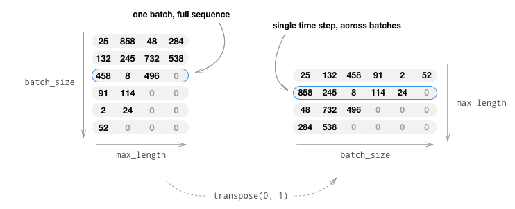
使用小批量还意味着我们必须注意批次中句子长度的变化。为了适应具有不同长度的句子在同一批次,我们将制作一个形状为 (max_length, batch_size) 的分批输入张量,其中比 max_length 短的句子会在 EOS_token 后填充为零。
如果我们通过转换单词为索引(indexesFromSentence)并填充零来将英文句子简单地转换为张量,我们的张量将具有 (batch_size, max_length) 的形状,并按第一维度索引会返回跨所有时间步的一整条序列。然而,我们需要能够沿着时间步并跨批次中的所有序列对批次进行索引。因此,我们将输入批量形状转置为 (max_length, batch_size),以便沿第一维度索引时可以返回批次中所有句子在某个时间步的值。我们在 zeroPadding 函数中隐式处理了这种转置。
inputVar 函数处理将句子转化为张量的过程,最终会生成一个形状正确的零填充张量。该函数还会返回每个序列的 lengths 张量,这些张量稍后会被传递给我们的解码器。
outputVar 函数执行与 inputVar 类似的功能,但它返回的不是 lengths 张量,而是一个二值掩码张量和最大目标句子长度。二值掩码张量的形状与目标输出张量相同,但每个元素中是 PAD_token 的地方值为 0,其他地方值为 1。
batch2TrainData 简单地接收一批对,并使用前述的函数返回输入和目标张量。
def indexesFromSentence(voc, sentence):
    return [voc.word2index[word] for word in sentence.split(' ')] + [EOS_token]


def zeroPadding(l, fillvalue=PAD_token):
    return list(itertools.zip_longest(*l, fillvalue=fillvalue))

def binaryMatrix(l, value=PAD_token):
    m = []
    for i, seq in enumerate(l):
        m.append([])
        for token in seq:
            if token == PAD_token:
                m[i].append(0)
            else:
                m[i].append(1)
    return m

# Returns padded input sequence tensor and lengths
def inputVar(l, voc):
    indexes_batch = [indexesFromSentence(voc, sentence) for sentence in l]
    lengths = torch.tensor([len(indexes) for indexes in indexes_batch])
    padList = zeroPadding(indexes_batch)
    padVar = torch.LongTensor(padList)
    return padVar, lengths

# Returns padded target sequence tensor, padding mask, and max target length
def outputVar(l, voc):
    indexes_batch = [indexesFromSentence(voc, sentence) for sentence in l]
    max_target_len = max([len(indexes) for indexes in indexes_batch])
    padList = zeroPadding(indexes_batch)
    mask = binaryMatrix(padList)
    mask = torch.BoolTensor(mask)
    padVar = torch.LongTensor(padList)
    return padVar, mask, max_target_len

# Returns all items for a given batch of pairs
def batch2TrainData(voc, pair_batch):
    pair_batch.sort(key=lambda x: len(x[0].split(" ")), reverse=True)
    input_batch, output_batch = [], []
    for pair in pair_batch:
        input_batch.append(pair[0])
        output_batch.append(pair[1])
    inp, lengths = inputVar(input_batch, voc)
    output, mask, max_target_len = outputVar(output_batch, voc)
    return inp, lengths, output, mask, max_target_len


# Example for validation
small_batch_size = 5
batches = batch2TrainData(voc, [random.choice(pairs) for _ in range(small_batch_size)])
input_variable, lengths, target_variable, mask, max_target_len = batches

print("input_variable:", input_variable)
print("lengths:", lengths)
print("target_variable:", target_variable)
print("mask:", mask)
print("max_target_len:", max_target_len)
定义模型
Seq2Seq 模型
我们聊天机器人的大脑是一个序列到序列 (seq2seq) 模型。seq2seq 模型的目标是以固定大小的模型为基础,接收一个可变长度的输入序列,并返回一个可变长度的输出序列。
Sutskever 等人的发现 表明,通过使用两个独立的循环神经网络(RNN),可以完成这项任务。一个 RNN 充当 编码器,将可变长度的输入序列编码为一个固定长度的上下文向量。理论上,这个上下文向量(RNN 的最终隐藏层)将包含关于输入给机器人的查询句子的语义信息。第二个 RNN 是 解码器,它接收一个输入单词和上下文向量,并返回序列中下一个单词的预测以及下一次迭代中使用的隐藏状态。
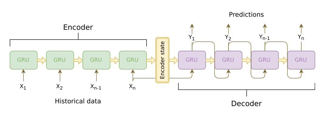
图片来源:https://jeddy92.github.io/JEddy92.github.io/ts_seq2seq_intro/
编码器
编码器 RNN 通过输入句子逐个标记(例如:单词)进行迭代,在每个时间步输出一个“输出”向量和一个“隐藏状态”向量。隐藏状态向量随后传递到下一时间步,而输出向量被记录下来。编码器将它在序列中各点看到的上下文转换为一个高维空间中的一组点,解码器将使用这些点来为给定任务生成有意义的输出。
我们的编码器核心是一个多层门控循环单元 (GRU),该单元由 Cho 等人在 2014 年发明。我们将使用 GRU 的双向变体,这意味着实际上有两个独立的 RNN:一个以正常顺序接收输入序列,另一个以反向顺序接收输入序列。两个网络的输出在每个时间步相加。使用双向 GRU 将使我们能够编码过去和未来的上下文。
双向 RNN:
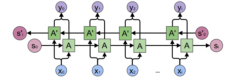
图片来源:https://colah.github.io/posts/2015-09-NN-Types-FP/
需要注意的是,“嵌入”层用于将单词索引编码到任意大小的特征空间中。对于我们的模型,此层将每个单词映射到大小为 hidden_size 的特征空间中。在训练后,这些值应编码相似意义单词之间的语义相似性。
最后,如果将填充过的批次序列传递到 RNN 模块中,则必须使用 nn.utils.rnn.pack_padded_sequence 和 nn.utils.rnn.pad_packed_sequence 分别对 RNN 过程中的填充值进行打包和解包。
计算图:
将单词索引转换为嵌入。
为 RNN 模块打包填充过的批次序列。
通过 GRU 的前向传播。
解包填充值。
对双向 GRU 的输出求和。
返回输出和最终的隐藏状态。
输入:
input_seq:输入句子的批次;形状=(max_length, batch_size)input_lengths:对应批次中每个句子的句子长度列表;形状=(batch_size)hidden:隐藏状态;形状=(n_layers x num_directions, batch_size, hidden_size)
输出:
outputs:GRU 最后一层隐藏层的输出特征(双向输出的总和);形状=(max_length, batch_size, hidden_size)hidden:GRU 更新后的隐藏状态;形状=(n_layers x num_directions, batch_size, hidden_size)
class EncoderRNN(nn.Module):
    def __init__(self, hidden_size, embedding, n_layers=1, dropout=0):
        super(EncoderRNN, self).__init__()
        self.n_layers = n_layers
        self.hidden_size = hidden_size
        self.embedding = embedding

        # Initialize GRU; the input_size and hidden_size parameters are both set to 'hidden_size'
        #   because our input size is a word embedding with number of features == hidden_size
        self.gru = nn.GRU(hidden_size, hidden_size, n_layers,
                          dropout=(0 if n_layers == 1 else dropout), bidirectional=True)

    def forward(self, input_seq, input_lengths, hidden=None):
        # Convert word indexes to embeddings
        embedded = self.embedding(input_seq)
        # Pack padded batch of sequences for RNN module
        packed = nn.utils.rnn.pack_padded_sequence(embedded, input_lengths)
        # Forward pass through GRU
        outputs, hidden = self.gru(packed, hidden)
        # Unpack padding
        outputs, _ = nn.utils.rnn.pad_packed_sequence(outputs)
        # Sum bidirectional GRU outputs
        outputs = outputs[:, :, :self.hidden_size] + outputs[:, : ,self.hidden_size:]
        # Return output and final hidden state
        return outputs, hidden
解码器
解码器 RNN 以逐标记的方式生成响应句子。它使用编码器的上下文向量和内部隐藏状态生成序列中的下一个单词,直到其输出一个 EOS_token,表示句子的结束。一个普通 seq2seq 解码器的常见问题是,如果我们仅依赖上下文向量来编码整个输入序列的语义,很可能会导致信息丢失。尤其是在处理长输入序列时,这将极大地限制解码器的能力。
为了解决这一问题,Bahdanau 等人 创建了一种“注意力机制”,使解码器能够集中关注输入序列的某些部分,而不是在每一步都使用整个固定上下文。
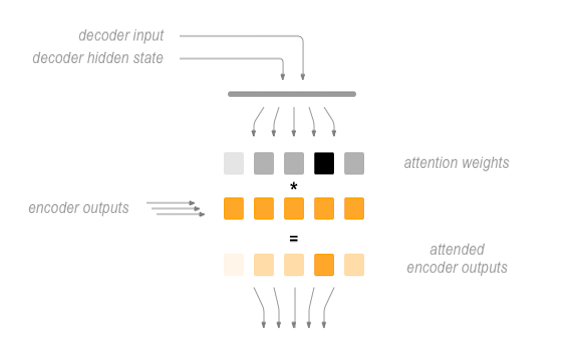
从高层次来看,注意力是利用解码器的当前隐藏状态和编码器的输出进行计算的。输出的注意力权重与输入序列具有相同的形状,允许我们将它们与编码器输出相乘,得到加权求和,这表明了要集中注意的编码器输出部分。Sean Robertson’s 的图很好地说明了这一点:
Luong 等人 在 Bahdanau 等人的基础上进行了改进,创建了“全局注意力”。主要区别在于,“全局注意力”考虑编码器的所有隐藏状态,而 Bahdanau 等人的“局部注意力”仅考虑编码器在当前时间步的隐藏状态。另一个区别是,在“全局注意力”中,我们仅使用来自当前时间步的解码器隐藏状态计算注意力权重或能量值。而 Bahdanau 等人的注意力计算需要了解解码器从上一个时间步的状态。此外,Luong 等人提供了各种方法来计算编码器输出和解码器输出之间的注意力能量值,这些称为“评分函数”:
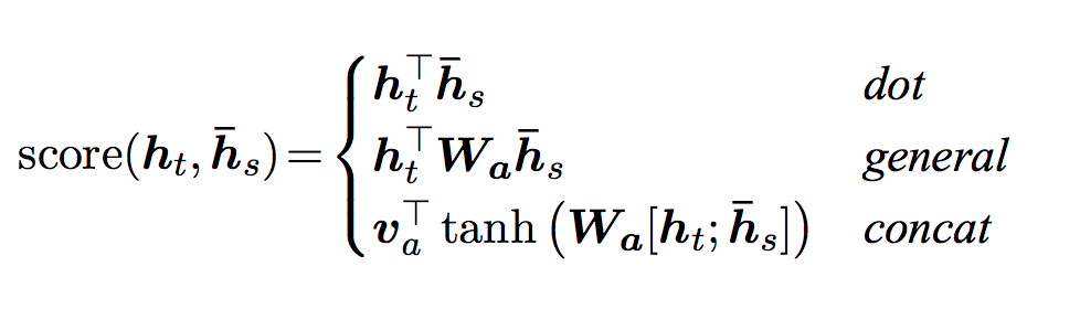
其中 \(h_t\) = 当前目标解码器状态,\(\bar{h}_s\) = 所有编码器状态。
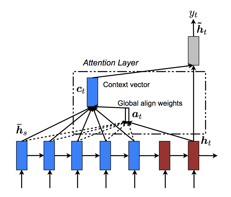
总体来说,全局注意力机制可以用以下图总结。需要注意的是,我们将实现“注意力层”作为一个独立的 nn.Module,称为 Attn。此模块的输出是一个形状为 (batch_size, 1, max_length) 的 softmax 归一化权重张量。
# Luong attention layer
class Attn(nn.Module):
    def __init__(self, method, hidden_size):
        super(Attn, self).__init__()
        self.method = method
        if self.method not in ['dot', 'general', 'concat']:
            raise ValueError(self.method, "is not an appropriate attention method.")
        self.hidden_size = hidden_size
        if self.method == 'general':
            self.attn = nn.Linear(self.hidden_size, hidden_size)
        elif self.method == 'concat':
            self.attn = nn.Linear(self.hidden_size * 2, hidden_size)
            self.v = nn.Parameter(torch.FloatTensor(hidden_size))

    def dot_score(self, hidden, encoder_output):
        return torch.sum(hidden * encoder_output, dim=2)

    def general_score(self, hidden, encoder_output):
        energy = self.attn(encoder_output)
        return torch.sum(hidden * energy, dim=2)

    def concat_score(self, hidden, encoder_output):
        energy = self.attn(torch.cat((hidden.expand(encoder_output.size(0), -1, -1), encoder_output), 2)).tanh()
        return torch.sum(self.v * energy, dim=2)

    def forward(self, hidden, encoder_outputs):
        # Calculate the attention weights (energies) based on the given method
        if self.method == 'general':
            attn_energies = self.general_score(hidden, encoder_outputs)
        elif self.method == 'concat':
            attn_energies = self.concat_score(hidden, encoder_outputs)
        elif self.method == 'dot':
            attn_energies = self.dot_score(hidden, encoder_outputs)

        # Transpose max_length and batch_size dimensions
        attn_energies = attn_energies.t()

        # Return the softmax normalized probability scores (with added dimension)
        return F.softmax(attn_energies, dim=1).unsqueeze(1)
现在我们已经定义了注意力子模块,可以实现实际的解码器模型了。对于解码器,我们将手动一次处理一个时间步的批次。这意味着我们的嵌入单词张量和 GRU 输出都将具有形状 (1, batch_size, hidden_size)。
计算图:
获取当前输入单词的嵌入。
通过单向 GRU 的前向传播。
计算来自 (2) 的当前 GRU 输出的注意力权重。
将注意力权重与编码器输出相乘,以获取新的“加权求和”上下文向量。
使用 Luong 方程 5 将加权上下文向量和 GRU 输出连接起来。
使用 Luong 方程 6(没有 softmax)预测下一个单词。
返回输出和最终的隐藏状态。
输入:
input_step:输入序列批次中的一个时间步(一个单词);形状=(1, batch_size)last_hidden:GRU 最后一层隐藏层;形状=(n_layers x num_directions, batch_size, hidden_size)encoder_outputs:编码器模型的输出;形状=(max_length, batch_size, hidden_size)
输出:
output:softmax 归一化张量,给出每个单词作为解码序列中正确下一个单词的概率;形状=(batch_size, voc.num_words)hidden:GRU 最终的隐藏状态;形状=(n_layers x num_directions, batch_size, hidden_size)
class LuongAttnDecoderRNN(nn.Module):
    def __init__(self, attn_model, embedding, hidden_size, output_size, n_layers=1, dropout=0.1):
        super(LuongAttnDecoderRNN, self).__init__()

        # Keep for reference
        self.attn_model = attn_model
        self.hidden_size = hidden_size
        self.output_size = output_size
        self.n_layers = n_layers
        self.dropout = dropout

        # Define layers
        self.embedding = embedding
        self.embedding_dropout = nn.Dropout(dropout)
        self.gru = nn.GRU(hidden_size, hidden_size, n_layers, dropout=(0 if n_layers == 1 else dropout))
        self.concat = nn.Linear(hidden_size * 2, hidden_size)
        self.out = nn.Linear(hidden_size, output_size)

        self.attn = Attn(attn_model, hidden_size)

    def forward(self, input_step, last_hidden, encoder_outputs):
        # Note: we run this one step (word) at a time
        # Get embedding of current input word
        embedded = self.embedding(input_step)
        embedded = self.embedding_dropout(embedded)
        # Forward through unidirectional GRU
        rnn_output, hidden = self.gru(embedded, last_hidden)
        # Calculate attention weights from the current GRU output
        attn_weights = self.attn(rnn_output, encoder_outputs)
        # Multiply attention weights to encoder outputs to get new "weighted sum" context vector
        context = attn_weights.bmm(encoder_outputs.transpose(0, 1))
        # Concatenate weighted context vector and GRU output using Luong eq. 5
        rnn_output = rnn_output.squeeze(0)
        context = context.squeeze(1)
        concat_input = torch.cat((rnn_output, context), 1)
        concat_output = torch.tanh(self.concat(concat_input))
        # Predict next word using Luong eq. 6
        output = self.out(concat_output)
        output = F.softmax(output, dim=1)
        # Return output and final hidden state
        return output, hidden
定义训练过程
掩码损失
由于我们处理的是带填充的序列批次,因此在计算损失时不能简单地考虑张量的所有元素。我们定义了 maskNLLLoss,以根据解码器的输出张量、目标张量和一个描述目标张量填充的二值掩码张量来计算损失。此损失函数计算掩码张量中值为 1 的元素的平均负对数似然。
def maskNLLLoss(inp, target, mask):
    nTotal = mask.sum()
    crossEntropy = -torch.log(torch.gather(inp, 1, target.view(-1, 1)).squeeze(1))
    loss = crossEntropy.masked_select(mask).mean()
    loss = loss.to(device)
    return loss, nTotal.item()
单次训练迭代
``train``函数包含单个训练迭代(单个输入批次)的算法。
我们将使用一些巧妙的技巧来帮助收敛:
第一个技巧是使用**教师强制**。这意味着,在由``teacher_forcing_ratio``设置的某种概率下,我们使用当前的目标词作为解码器的下一个输入,而不是使用解码器当前的预测。这种技术相当于给解码器戴上了辅助轮,有助于更高效地训练。然而,教师强制可能在推理时导致模型的不稳定性,因为训练期间解码器可能没有足够的机会生成自己的输出序列。因此,我们必须谨慎设置``teacher_forcing_ratio``,并且不要被快速收敛所迷惑。
我们实现的第二个技巧是**梯度裁剪**。这是一种常用的技术,用于应对“梯度爆炸”问题。本质上,通过将梯度裁剪或限制在一个最大值内,我们可以防止梯度指数增长,避免溢出(NaN)或在代价函数的陡峭区域过冲。
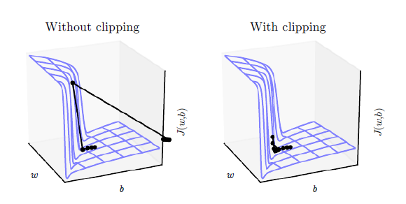
图片来源: Goodfellow et al. Deep Learning. 2016. https://www.deeplearningbook.org/
操作顺序:
通过编码器前向传播整个输入批次。
将解码器的输入初始化为SOS_token,隐状态初始化为编码器的最终隐状态。
将输入批次序列一次一步地传递给解码器。
如果使用教师强制:将当前目标设置为解码器的下一个输入;否则:将解码器的当前输出设置为下一个输入。
计算并累积损失。
执行反向传播。
裁剪梯度。
更新编码器和解码器模型参数。
备注
PyTorch的RNN模块(RNN,LSTM,GRU)可以像其他非递归层一样,简单地通过它们传递整个输入序列(或序列的批次)。我们在``encoder``中以这种方式使用了``GRU``层。实际上,在底层,这是一种迭代过程,循环遍历每个时间步计算隐状态。或者,你可以一次一步地运行这些模块。在这种情况下,我们在训练过程中手动循环序列,就像对``decoder``模型所做的一样。只要你正确理解这些模块的概念模型,实现序列模型就会非常简单。
def train(input_variable, lengths, target_variable, mask, max_target_len, encoder, decoder, embedding,
          encoder_optimizer, decoder_optimizer, batch_size, clip, max_length=MAX_LENGTH):

    # Zero gradients
    encoder_optimizer.zero_grad()
    decoder_optimizer.zero_grad()

    # Set device options
    input_variable = input_variable.to(device)
    target_variable = target_variable.to(device)
    mask = mask.to(device)
    # Lengths for RNN packing should always be on the CPU
    lengths = lengths.to("cpu")

    # Initialize variables
    loss = 0
    print_losses = []
    n_totals = 0

    # Forward pass through encoder
    encoder_outputs, encoder_hidden = encoder(input_variable, lengths)

    # Create initial decoder input (start with SOS tokens for each sentence)
    decoder_input = torch.LongTensor([[SOS_token for _ in range(batch_size)]])
    decoder_input = decoder_input.to(device)

    # Set initial decoder hidden state to the encoder's final hidden state
    decoder_hidden = encoder_hidden[:decoder.n_layers]

    # Determine if we are using teacher forcing this iteration
    use_teacher_forcing = True if random.random() < teacher_forcing_ratio else False

    # Forward batch of sequences through decoder one time step at a time
    if use_teacher_forcing:
        for t in range(max_target_len):
            decoder_output, decoder_hidden = decoder(
                decoder_input, decoder_hidden, encoder_outputs
            )
            # Teacher forcing: next input is current target
            decoder_input = target_variable[t].view(1, -1)
            # Calculate and accumulate loss
            mask_loss, nTotal = maskNLLLoss(decoder_output, target_variable[t], mask[t])
            loss += mask_loss
            print_losses.append(mask_loss.item() * nTotal)
            n_totals += nTotal
    else:
        for t in range(max_target_len):
            decoder_output, decoder_hidden = decoder(
                decoder_input, decoder_hidden, encoder_outputs
            )
            # No teacher forcing: next input is decoder's own current output
            _, topi = decoder_output.topk(1)
            decoder_input = torch.LongTensor([[topi[i][0] for i in range(batch_size)]])
            decoder_input = decoder_input.to(device)
            # Calculate and accumulate loss
            mask_loss, nTotal = maskNLLLoss(decoder_output, target_variable[t], mask[t])
            loss += mask_loss
            print_losses.append(mask_loss.item() * nTotal)
            n_totals += nTotal

    # Perform backpropagation
    loss.backward()

    # Clip gradients: gradients are modified in place
    _ = nn.utils.clip_grad_norm_(encoder.parameters(), clip)
    _ = nn.utils.clip_grad_norm_(decoder.parameters(), clip)

    # Adjust model weights
    encoder_optimizer.step()
    decoder_optimizer.step()

    return sum(print_losses) / n_totals
训练迭代
现在终于可以将完整的训练过程与数据结合起来了。``trainIters``函数负责在传递的模型、优化器、数据等基础上运行``n_iterations``次训练。该函数非常直观,因为我们已经用``train``函数完成了主要工作。
需要注意的一点是,当我们保存我们的模型时,我们保存了一个包含编码器和解码器``state_dicts``(参数)的压缩包,优化器的``state_dicts``,损失,迭代等。以这种方式保存模型将为我们提供最大的灵活性来使用检查点。加载检查点后,我们可以使用模型参数运行推理,或者从我们中断的地方继续训练。
def trainIters(model_name, voc, pairs, encoder, decoder, encoder_optimizer, decoder_optimizer, embedding, encoder_n_layers, decoder_n_layers, save_dir, n_iteration, batch_size, print_every, save_every, clip, corpus_name, loadFilename):

    # Load batches for each iteration
    training_batches = [batch2TrainData(voc, [random.choice(pairs) for _ in range(batch_size)])
                      for _ in range(n_iteration)]

    # Initializations
    print('Initializing ...')
    start_iteration = 1
    print_loss = 0
    if loadFilename:
        start_iteration = checkpoint['iteration'] + 1

    # Training loop
    print("Training...")
    for iteration in range(start_iteration, n_iteration + 1):
        training_batch = training_batches[iteration - 1]
        # Extract fields from batch
        input_variable, lengths, target_variable, mask, max_target_len = training_batch

        # Run a training iteration with batch
        loss = train(input_variable, lengths, target_variable, mask, max_target_len, encoder,
                     decoder, embedding, encoder_optimizer, decoder_optimizer, batch_size, clip)
        print_loss += loss

        # Print progress
        if iteration % print_every == 0:
            print_loss_avg = print_loss / print_every
            print("Iteration: {}; Percent complete: {:.1f}%; Average loss: {:.4f}".format(iteration, iteration / n_iteration * 100, print_loss_avg))
            print_loss = 0

        # Save checkpoint
        if (iteration % save_every == 0):
            directory = os.path.join(save_dir, model_name, corpus_name, '{}-{}_{}'.format(encoder_n_layers, decoder_n_layers, hidden_size))
            if not os.path.exists(directory):
                os.makedirs(directory)
            torch.save({
                'iteration': iteration,
                'en': encoder.state_dict(),
                'de': decoder.state_dict(),
                'en_opt': encoder_optimizer.state_dict(),
                'de_opt': decoder_optimizer.state_dict(),
                'loss': loss,
                'voc_dict': voc.__dict__,
                'embedding': embedding.state_dict()
            }, os.path.join(directory, '{}_{}.tar'.format(iteration, 'checkpoint')))
定义评估
在训练完模型后,我们希望能够亲自与机器人交谈。首先,我们必须定义如何将模型解码为编码输入。
贪心解码
贪心解码是训练时**不**使用教师强制时的解码方法。换句话说,对于每个时间步,我们简单地从``decoder_output``中选择softmax值最高的词语。该解码方法在单个时间步层面是最优的。
为了方便贪心解码操作,我们定义了一个``GreedySearchDecoder``类。当运行时,此类的对象接收一个形状为*(input_seq length, 1)*的输入序列(input_seq),一个标量输入长度(input_length)张量,以及一个``max_length``来限制响应句子的长度。输入句子通过以下计算图进行评估:
计算图:
通过编码器模型前向传播输入。
准备编码器最终的隐层作为解码器的第一个隐状态输入。
将解码器的第一个输入初始化为SOS_token。
初始化张量以附加解码后的词语。
- 逐字解码,一个时间步一个时间步地进行:
通过解码器前向传播。
获取最可能的词语标记及其softmax分数。
记录标记和分数。
准备当前标记作为解码器的下一个输入。
返回词语标记和分数的集合。
class GreedySearchDecoder(nn.Module):
    def __init__(self, encoder, decoder):
        super(GreedySearchDecoder, self).__init__()
        self.encoder = encoder
        self.decoder = decoder

    def forward(self, input_seq, input_length, max_length):
        # Forward input through encoder model
        encoder_outputs, encoder_hidden = self.encoder(input_seq, input_length)
        # Prepare encoder's final hidden layer to be first hidden input to the decoder
        decoder_hidden = encoder_hidden[:self.decoder.n_layers]
        # Initialize decoder input with SOS_token
        decoder_input = torch.ones(1, 1, device=device, dtype=torch.long) * SOS_token
        # Initialize tensors to append decoded words to
        all_tokens = torch.zeros([0], device=device, dtype=torch.long)
        all_scores = torch.zeros([0], device=device)
        # Iteratively decode one word token at a time
        for _ in range(max_length):
            # Forward pass through decoder
            decoder_output, decoder_hidden = self.decoder(decoder_input, decoder_hidden, encoder_outputs)
            # Obtain most likely word token and its softmax score
            decoder_scores, decoder_input = torch.max(decoder_output, dim=1)
            # Record token and score
            all_tokens = torch.cat((all_tokens, decoder_input), dim=0)
            all_scores = torch.cat((all_scores, decoder_scores), dim=0)
            # Prepare current token to be next decoder input (add a dimension)
            decoder_input = torch.unsqueeze(decoder_input, 0)
        # Return collections of word tokens and scores
        return all_tokens, all_scores
评估我的文本
现在既然我们定义了解码方法,我们可以编写函数来评估字符串输入句子。evaluate``函数管理处理输入句子的底层过程。我们首先将句子格式化为由*batch_size==1*组成的单词索引输入批次。对此,我们将句子的单词转换为对应的索引值,并转置张量的维度以适应我们的模型。我们还创建了一个``lengths``张量,包含我们输入句子的长度。在这种情况下,由于我们一次仅评估一个句子(``batch_size==1),lengths``是标量。接下来,我们使用我们的``GreedySearchDecoder``对象(``searcher)获取解码后的响应句子张量。最后,我们将响应的索引值转换成单词并返回解码后单词的列表。
``evaluateInput``充当我们聊天机器人的用户界面。当被调用时,将弹出一个输入文本字段,我们可以在其中输入查询句子。在输入句子并按下*Enter*后,我们的文本会以与训练数据相同的方式进行规范化,并最终被传递给``evaluate``函数以获得解码后的输出句子。我们循环此过程,因此可以继续与机器人聊天,直到输入“q”或“quit”。
最后,如果输入的句子中包含词汇表中没有的单词,我们会通过打印一条错误信息并提示用户输入另一个句子来优雅地处理。
def evaluate(encoder, decoder, searcher, voc, sentence, max_length=MAX_LENGTH):
    ### Format input sentence as a batch
    # words -> indexes
    indexes_batch = [indexesFromSentence(voc, sentence)]
    # Create lengths tensor
    lengths = torch.tensor([len(indexes) for indexes in indexes_batch])
    # Transpose dimensions of batch to match models' expectations
    input_batch = torch.LongTensor(indexes_batch).transpose(0, 1)
    # Use appropriate device
    input_batch = input_batch.to(device)
    lengths = lengths.to("cpu")
    # Decode sentence with searcher
    tokens, scores = searcher(input_batch, lengths, max_length)
    # indexes -> words
    decoded_words = [voc.index2word[token.item()] for token in tokens]
    return decoded_words


def evaluateInput(encoder, decoder, searcher, voc):
    input_sentence = ''
    while(1):
        try:
            # Get input sentence
            input_sentence = input('> ')
            # Check if it is quit case
            if input_sentence == 'q' or input_sentence == 'quit': break
            # Normalize sentence
            input_sentence = normalizeString(input_sentence)
            # Evaluate sentence
            output_words = evaluate(encoder, decoder, searcher, voc, input_sentence)
            # Format and print response sentence
            output_words[:] = [x for x in output_words if not (x == 'EOS' or x == 'PAD')]
            print('Bot:', ' '.join(output_words))

        except KeyError:
            print("Error: Encountered unknown word.")
运行模型
最后,到了运行模型的时候了!
无论我们是想训练还是测试聊天机器人模型,都必须初始化单独的编码器和解码器模型。在以下代码块中,我们设置了所需的配置,选择从头开始或设置一个检查点进行加载,并构建和初始化模型。可以自由尝试不同的模型配置以优化性能。
# Configure models
model_name = 'cb_model'
attn_model = 'dot'
#``attn_model = 'general'``
#``attn_model = 'concat'``
hidden_size = 500
encoder_n_layers = 2
decoder_n_layers = 2
dropout = 0.1
batch_size = 64

# Set checkpoint to load from; set to None if starting from scratch
loadFilename = None
checkpoint_iter = 4000
从检查点加载的示例代码:
loadFilename = os.path.join(save_dir, model_name, corpus_name,
                    '{}-{}_{}'.format(encoder_n_layers, decoder_n_layers, hidden_size),
                    '{}_checkpoint.tar'.format(checkpoint_iter))
# Load model if a ``loadFilename`` is provided
if loadFilename:
    # If loading on same machine the model was trained on
    checkpoint = torch.load(loadFilename)
    # If loading a model trained on GPU to CPU
    #checkpoint = torch.load(loadFilename, map_location=torch.device('cpu'))
    encoder_sd = checkpoint['en']
    decoder_sd = checkpoint['de']
    encoder_optimizer_sd = checkpoint['en_opt']
    decoder_optimizer_sd = checkpoint['de_opt']
    embedding_sd = checkpoint['embedding']
    voc.__dict__ = checkpoint['voc_dict']


print('Building encoder and decoder ...')
# Initialize word embeddings
embedding = nn.Embedding(voc.num_words, hidden_size)
if loadFilename:
    embedding.load_state_dict(embedding_sd)
# Initialize encoder & decoder models
encoder = EncoderRNN(hidden_size, embedding, encoder_n_layers, dropout)
decoder = LuongAttnDecoderRNN(attn_model, embedding, hidden_size, voc.num_words, decoder_n_layers, dropout)
if loadFilename:
    encoder.load_state_dict(encoder_sd)
    decoder.load_state_dict(decoder_sd)
# Use appropriate device
encoder = encoder.to(device)
decoder = decoder.to(device)
print('Models built and ready to go!')
运行训练
如果想要训练模型,请运行以下代码块。
首先,我们设置训练参数,然后初始化优化器,最后调用``trainIters``函数运行训练迭代。
# Configure training/optimization
clip = 50.0
teacher_forcing_ratio = 1.0
learning_rate = 0.0001
decoder_learning_ratio = 5.0
n_iteration = 4000
print_every = 1
save_every = 500

# Ensure dropout layers are in train mode
encoder.train()
decoder.train()

# Initialize optimizers
print('Building optimizers ...')
encoder_optimizer = optim.Adam(encoder.parameters(), lr=learning_rate)
decoder_optimizer = optim.Adam(decoder.parameters(), lr=learning_rate * decoder_learning_ratio)
if loadFilename:
    encoder_optimizer.load_state_dict(encoder_optimizer_sd)
    decoder_optimizer.load_state_dict(decoder_optimizer_sd)

# If you have an accelerator, configure it to call
for state in encoder_optimizer.state.values():
    for k, v in state.items():
        if isinstance(v, torch.Tensor):
            state[k] = v.to(device)

for state in decoder_optimizer.state.values():
    for k, v in state.items():
        if isinstance(v, torch.Tensor):
            state[k] = v.to(device)

# Run training iterations
print("Starting Training!")
trainIters(model_name, voc, pairs, encoder, decoder, encoder_optimizer, decoder_optimizer,
           embedding, encoder_n_layers, decoder_n_layers, save_dir, n_iteration, batch_size,
           print_every, save_every, clip, corpus_name, loadFilename)
运行评估
要与模型聊天,请运行以下代码块。
# Set dropout layers to ``eval`` mode
encoder.eval()
decoder.eval()

# Initialize search module
searcher = GreedySearchDecoder(encoder, decoder)

# Begin chatting (uncomment and run the following line to begin)
# evaluateInput(encoder, decoder, searcher, voc)
总结
这就是本教程的全部内容了。恭喜你,现在你已经了解了构建生成式聊天机器人模型的基本知识!如果感兴趣,可以通过调整模型和训练参数以及自定义用于训练模型的数据来尝试改变聊天机器人的行为。
查看其他教程,了解更多关于PyTorch的酷炫深度学习应用!
脚本总运行时间: (0 分钟 0.000 秒)
